top of page


Model Analysis
Data Cleaning
In order to properly run models, we need to clean the data so that it is in a model friendly format. This means dropping unnecessary features, making features into ints and floats instead of strings, imputing or dropping missing data, generating dummy variables, and standardizing the data.
To start we made a function that tells us the amount of unique values a given column has. This helped us determine what should be made into dummy variables and what should be dropped.


We see that emp_title and title have too many values to create dummies for. So we should drop them. We should likely keep addr_state information as that could be relevant. Anything that has 2 unique values can be converted into a binary feature. Anything with more, we make dummies for. We do this for term as well because it can either be a short term loan or long term loan. The lists below that indicate the way these features need to be cleaned and are followed by their cleaning functions.


Helper Functions
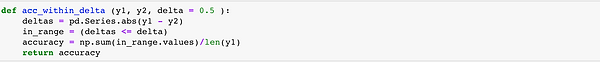
We built helper functions to 1. explore a slice of a dataframe 2. determine NaN prevalent features 3. calculate the accuracy of our predictions within a margin of error and 4. convert subgrades into numerical values that fit regression models.

Feature Selection
To focus our model on exploring how Lending Club appraises an application and then assigns it a grade, we had to eliminate all data that would not be submitted with the initial application, which meant dropping 121 feature variables. The spreadsheet below enumerates the features we initially kept, though those highlighted in red were only kept for data augmentation and were later dropped.


Data Augmentation
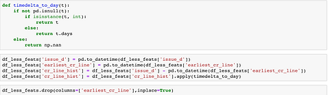
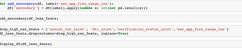
We created three new features variables: fico_avg, secondary, and cr_line_hist. We created fico_avg because the dataset provided a FICO score range instead. We created secondary as a binary variable to take into account the effect of a second signer on the application which happened around 4% of the time. Finally we created cr_line_hist to make the information conveyed by earliest_cr_line contextual and useful for our analysis. We also dropped all features with high NaN counts.
Data Prep
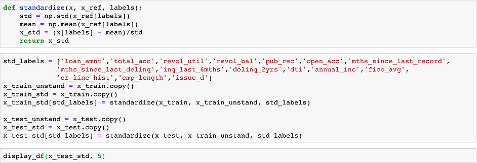
We handled some last loose ends, such as either dropping or imputing the last remaining NaN observations, before then splitting and standardizing our data. When we split our data into training and test sets, we stratified on sub_grade, so that an equal distribution of grades was present in both sets.

Models
We used a simple OLS regression as our baseline model and followed up with LASSO and Ridge regressions, a Logistic regression, a Decision Tree, and a Random Forest model. Our LASSO regression and Decision Tree models proved particularly insightful.
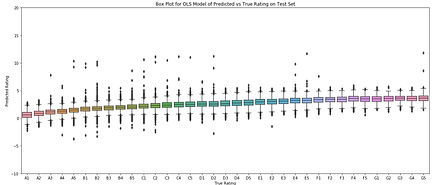
Baseline Model
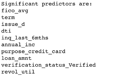
LASSO Model
Regularizing suppresses features and coefficient magnitudes, making it ideal for exploring how features stack up against one another and influence risk grade. We've presented a piece of that exploration below.


Ridge Model

Decision Tree Model


Random Forest Model


Logistic Regression

Summary
The most accurate model we made was the Decision Tree, able to predict an application's risk score within a letter grade with an accuracy of around 77%. The linear regression with Lasso regularization performed only slightly worse and offers the benefit of the linear regression coefficients which can be used to explain the relative importance of variables to a lay person. Therefore, we chose the Lasso results for the conclusions on our website.
Data Cleaning
Helper
Feature
Augmentation
Prep
Model
bottom of page